

Description:
Time series analysis and forecasting is an important area of statistics that deals with analyzing and forecasting the future behaviour of time series data. Time series data is data that is collected over a period of time, such as daily stock prices, monthly sales figures, or yearly weather records. Time series analysis and forecasting can be used to make predictions about the future behaviour of the data and to identify trends or patterns in the data.
In this guide, we will explore the basics of time series analysis and forecasting. We will cover topics such as ARIMA models, and more.
While working on the dataset, there are many factors that are relevant for time series analysis and forecasting.
- Trend: The overall direction of a time series (upward or downward).
- Seasonality: Short-term fluctuations that repeat in a regular pattern over time.
- Cyclicality: Long-term fluctuations that happen at a slower rate than seasonality.
- Autocorrelation: The degree to which the value of a variable at a given point in time is related to the value of the same variable at a previous point in time.
- Lags: The amount of time between two related points in a time series.
- Exogenous Variables: Variables outside of the time series that can have an influence on it.
- Outliers: Extreme values that can potentially have an outsized influence on a time series.
In this post, we will introduce different characteristics of time series and learn how we can model them to obtain accurate forecasts.
Video: – Time-Series data analysis
What is Stationarity?
Stationarity is an important characteristic of time series. Stationarity means that the statistical properties of a time series are constant over time. Stationarity allows us to make predictions and use certain statistical methods to analyze the data. Non-stationary time series can be more difficult to predict and analyze due to their varying characteristics.
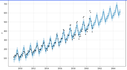
What is Seasonality?
Seasonality in a time series is the presence of regular patterns or periodic fluctuations of a given variable at specific times of the year. It is a characteristic of a time series and can be seen in most economic, financial and social phenomena. Seasonality is an important factor to consider when modeling and forecasting time series data.
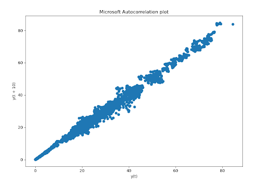
What is Autocorrelation?
Autocorrelation in time series is a measure of the similarity between values of a time series at different points in time. It is the correlation of a time series with its own offset values. Autocorrelation can be used to detect seasonality, trends, and other patterns in a time series. Autocorrelation can also be used to predict future values in a time series.
In this article, you will learn how to perform time series analysis using the ARIMA model.
ARIMA (Autoregressive Integrated Moving Average Model) Model
An ARIMA (Autoregressive Integrated Moving Average) model is a type of statistical model used in time series forecasting. It is a combination of autoregressive (AR) and moving average (MA) models that are used to predict future values based on past data. ARIMA models are used to analyze and forecast time-series data, such as stock prices, sales, inventory levels, and economic indicators.
ARIMA models are based on the assumption that future values are a linear combination of past values and random noise. The model is designed to capture the autocorrelation of the data, which is the correlation between the current value and the previous values.
ARIMA models use three parameters (p, d, q) to identify the order of the AR and MA components. The “p” parameter is the order of the autoregressive component, the “d” parameter is the order of the differencing component, and the “q” parameter is the order of the moving average component. The model is used to analyze the data and make predictions about future values.
A linear regression model is a type of statistical model used to examine the linear relationship between two or more variables. It is used to predict the value of one variable (dependent variable) based on the values of one or more other variables (independent variables).
A linear regression model assumes that the relationship between the dependent and independent variables is linear and that the error term is normally distributed. The model attempts to estimate the coefficients of the independent variables, which can then be used to make predictions about the dependent variable. The model can also be used to identify any non-linear relationships between the variables.

Video:- Time-Series data analysis
Coding Steps for Microsoft Stocks Time Series Analysis
Step 1. Import dependent libraries and functions for this project.
Step 2. Import data set of people’s income in panda dataframe.
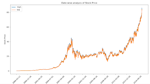
Step 3. Analyze the highest and lowest value of Microsoft stock price.
Output:
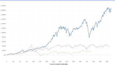
Step 4. Now, do a cumulative sum of all the indexes to find out the covariance of stock price with Time.
Output:
Note: In the above graph we can increase our graph with Time. So, covariance is positive with time.
Step 5. Now, split the data into train and test data.
Note: Now, plot the graph for test and train data.
Step 6. Define the function to compare “y_predictaed” value and “y_true” value.
Step 7. Store day open stock price value with train and test data.
Step 8. Extract train data in the history list also you can create an empty list for prediction values.
Step 9. Forecast Price with Arima Algorithm
Step 10. Now, fit the model and forecast the values in the for loop.
Step 11. After the forecast stock prices of Microsoft, find out the mean square error.
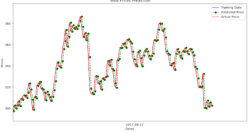
Step 12. Now, plot the graph b/w Actual test data and Predicted test data.
Output:
Conclusion:
With this, we have come to the end of this article. Hope it was insightful for you and made you learn about time series analysis and forecasting.

Leave A Comment
Related Posts
Coding is generally considered a boring activity. After all, who wants to sit in front of a computer all day writing in a language that can’t even be read? But that is not all there is to code. It can be used for some really fun coding facts stuff, and there is so much amazing work that you can do only if you knew how to code.
5 Coding Facts That Blow Your Mind
Let us look at five great fun coding facts you might not know about coding.
You Can Make Games With Code
Coding is an umbrella term for the scores of languages and their versions that programmers use to make their applications. We have all played games, on consoles, our mobile phones, or our desktop computers and laptops, at some point in our life. It might not surprise you to know that these games are also created using code. The complex physics of the characters in these games, the design of the environment of the games, and each minute movement in the games have a piece of code behind them.
Game designers typically write in languages such as C++, C#, and Java. These are also some of the most popular kids coding languages, especially for children who like gaming. Coding courses are available widely in all of these languages and the broad domain of game design.
You Do Better At School If You Code
Making games and indulging in the fun applications of coding is all fine, but coding can have great advantages at school as well. Once you start taking classes that teach coding for kids, you will realize that coding requires a lot of brainpower as well. Coding even for the most fun tasks requires you to think quite a bit, and this sharpens your mind and increases your capability to think logically.
This logical capability can be of a lot of use to you at school. Especially in subjects like mathematics, you might find yourself topping the class simply because of the practice you got during coding! In fact, coding and mathematics have a kind of symbiotic relationship – what you learn in maths comes of use in code and vice versa.
You Can Follow Your Interest Using Coding
Regardless of what your favorite subject is, or what fields you are interested in, you will find a use for code everywhere. Be it through developing software, creating an all-new app, making a game, or building a simple utility, you will find that coding facts can be a way to enable you to follow your interests through a different path.
All subjects from science to social studies and from mathematics to philosophy use coding in some way for research or education. Be it sports or music, art or architecture, utilities that are made using code are prevalent in every field that you can think of. Taking simple online coding courses can qualify you and build your interest in creating such utilities.
You Can Predict Future Events Through Code
Did you know that predicting the future is an application of coding! Predictive modeling is a field of programming in which code is used to try and predict what will happen in the future on the basis of events that took place in the past. It uses concepts of artificial intelligence and machine learning to create algorithms that learn the behavior of past data and determine the course of future data.
Predictive modeling is one of the most futuristic applications of code and is used to determine everything from the next movie you will like on Netflix to whether it will rain tomorrow. You can opt for closing classes in machine learning to know more about the field, and create your own utilities to predict the future!
Coding Is Free!
You don’t need any sophisticated apparatus except your laptop for coding. All you need is the will to learn more and follow your interests through code. To learn to code you do not need to go to a special school or have any special capabilities. You can opt for free coding classes for kids which are held completely online and follow a completely hands-off approach in helping kids learn to code. There are also a vast number of coding sites for kids on which they can log in to learn basic coding facts for kids without even having to enroll in a class.
Conclusion
The future is already being written, and it is being written in code. Coding for kids classes can help kids of all ages currently going to school not just learn to code but also to have fun in the process. The above applications of code can be a major stepping stone to build the interest of kids in coding, after which they can hone their interests and new skills on even more advanced applications. A platform such as Learningbix can be an excellent way for you to get started.